Example script illustrating the stimuli

Contents

Load in the stimuli

% load in the stimuli
load('stimuli.mat');

% check the workspace
whos

  Name            Size                  Bytes  Class     Attributes

  bpfilter       21x21                   3528  double              
  conimages       1x260             247497712  cell                
  images          1x260            1664909120  cell                

Inspect the stimuli

% look at one of the stimulus frames
figure;
imagesc(double(images{12}(:,:,1)));
axis equal tight;
colorbar;
title('Stimulus frame');

% write out the first frame of each stimulus
whframe = 1;  % which index to write out
res = 256;    % downsample to what resolution
mkdir('thumbnails');
for p=1:length(images)
  imwrite(uint8(imresize(double(images{p}(:,:,whframe)),[res res])), ...
          sprintf('thumbnails/thumbnails%03d.png',p));
end

Warning: Directory already exists. 

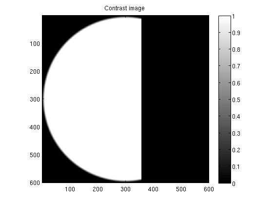
Inspect the contrast images

% look at one of the contrast images
figure;
imagesc(double(conimages{12}));
axis equal tight;
colorbar;
title('Contrast image');

% write out each contrast image
res = 256;  % downsample to what resolution
mkdir('conimages');
for p=1:length(conimages)
  if ~isempty(conimages{p})
    imwrite(uint8(255*imresize(conimages{p},[res res])), ...
            sprintf('conimages/conimages%03d.png',p));
  end
end

Warning: Directory already exists. 

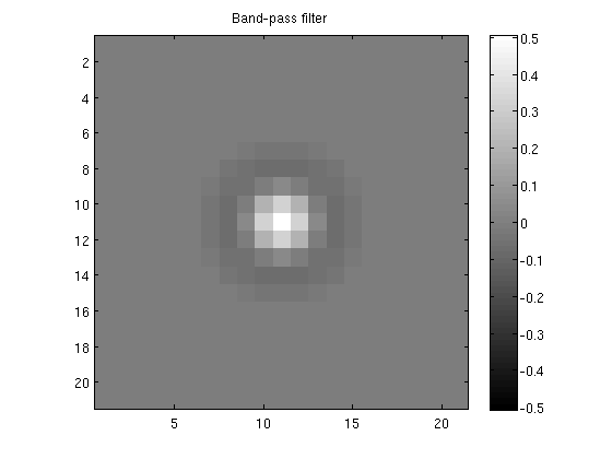
Inspect the band-pass filter

% look at the band-pass filter that was used to construct some of the stimuli
% in stimulus sets 2 and 3
mx = max(abs(bpfilter(:)));
figure;
imagesc(bpfilter,[-mx mx]);
axis equal tight;
colorbar;
title('Band-pass filter');

% now, let's look at the filter in the Fourier domain.

% first, let's define some constants
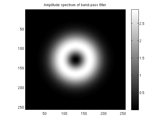
res = 256;   % the stimuli were constructed at a resolution of 256 x 256
fov = 12.7;  % on average, the stimuli occupied 12.7 x 12.7 degrees of visual angle

% place filter in a full-sized image
temp = zeros(res,res);
temp(1:size(bpfilter,1),1:size(bpfilter,2)) = bpfilter;

% compute the amplitude spectrum
temp = fftshift(abs(fft2(temp)));

% visualize the amplitude spectrum
figure;
imagesc(temp);
axis equal tight;
colorbar;
title('Amplitude spectrum of band-pass filter');

% visualize a profile through the amplitude spectrum
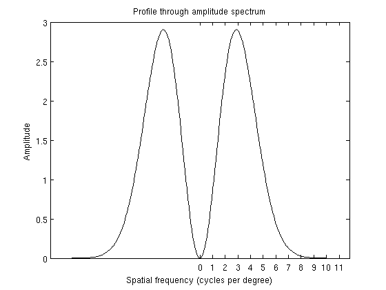
figure;
plot(-res/2:res/2-1,temp(res/2+1,:),'k-');
cpd = 0:20;  % cycles per degree to put tick marks at
set(gca,'XTick',cpd*fov,'XTickLabel',cpd);
xlabel('Spatial frequency (cycles per degree)');
ylabel('Amplitude');
title('Profile through amplitude spectrum');

Published with MATLAB® 7.9