Example script illustrating how to fit the SOC model

Contents

Note

% This script assumes familiarity with the script that
% illustrates how to fit the CSS model (cssmodel_example.m).

Add code to the MATLAB path

addpath(genpath(fullfile(pwd,'code')));

Load data

% load data from the third dataset
load('dataset03.mat','betamn','betase');

Load stimuli

load('stimuli.mat','images');

Perform stimulus pre-processing (Part 1)

% extract the stimuli we need and then concatenate along the third dimension.
% (note that we fit only the first 99 (out of 156) stimuli;
% this corresponds to what was done in the paper.)
stimulus = images(69+(1:99));
stimulus = cat(3,stimulus{:});
clear images;

% resize the stimuli to 150 x 150 to reduce computational time.
% use single-format to save memory.
temp = zeros(150,150,size(stimulus,3),'single');
for p=1:size(stimulus,3)
  temp(:,:,p) = imresize(single(stimulus(:,:,p)),[150 150],'cubic');
end
stimulus = temp;
clear temp;

% ensure that all values are between 0 and 254.
% rescale values to the range [0,1].
% subtract off the background luminance (0.5).
% after these steps, all pixel values will be in the
% range [-.5,.5] with the background corresponding to 0.
stimulus(stimulus < 0) = 0;
stimulus(stimulus > 254) = 254;
stimulus = stimulus/254 - 0.5;

% pad the stimulus with zeros (to reduce edge effects).
% the new resolution is 180 x 180 (15-pixel padding on each side).
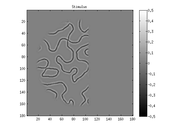
stimulus = placematrix(zeros(180,180,size(stimulus,3),'single'),stimulus);

% inspect one of the stimuli
figure;
imagesc(stimulus(:,:,100));
axis image tight;
caxis([-.5 .5]);
colormap(gray);
colorbar;
title('Stimulus');

Perform stimulus pre-processing (Part 2)

% thus far, we have performed very basic pre-processing of the stimulus.  now,
% we will proceed to perform more specialized operations that can be considered
% to be a more integral part of the SOC model.  the reason that we consider these
% operations to be "pre-processing" is these operations come before the
% operations that we are primarily concerned with in this example script.
%
% essentially, the goal of this script is to fit certain model parameters; any
% pre-computations we can perform prior to the fitting of these parameters
% will help reduce computational time.

% apply Gabor filters to the stimuli.  filters occur at different positions,
% orientations, and phases.  there are several parameters that govern the
% design of the filters:
%   the number of cycles per image is 37.5*(180/150)
%   the spatial frequency bandwidth of the filters is 1 octave
%   the separation of adjacent filters is 1 std dev of the Gaussian envelopes
%     (this results in a 90 x 90 grid of positions)
%   filters occur at 8 orientations
%   filters occur at 2 phases (between 0 and pi)
%   the Gaussian envelopes are thresholded at .01
%   filters are scaled to have an equivalent Michelson contrast of 1
%   the dot-product between each filter and each stimulus is computed
% after this step, stimulus is images x phases*orientations*positions.
stimulus = applymultiscalegaborfilters(reshape(stimulus,180*180,[])', ...
  37.5*(180/150),-1,1,8,2,.01,2,0);

grid is 90 x 90, gbrsize is 14 (sd is 2.2486875016), indices is [1 3 5 7 9 11 13 15 17 19 21 23 25 27 29 31 33 35 37 39 41 43 45 47 49 51 53 55 57 59 61 63 65 67 69 71 73 75 77 79 81 83 85 87 89 91 93 95 97 99 101 103 105 107 109 111 113 115 117 119 121 123 125 127 129 131 133 135 137 139 141 143 145 147 149 151 153 155 157 159 161 163 165 167 169 171 173 175 177 179]

% compute the square root of the sum of the squares of the outputs of
% quadrature-phase filter pairs (this is the standard complex-cell energy model).
% after this step, stimulus is images x orientations*positions.
stimulus = sqrt(blob(stimulus.^2,2,2));

% compute the population term in the divisive-normalization equation.
% this term is simply the average across the complex-cell outputs
% at each position (averaging across orientation).
stimulusPOP = blob(stimulus,2,8)/8;

% repeat the population term for each of the orientations
stimulusPOP = upsamplematrix(stimulusPOP,8,2,[],'nearest');

% apply divisive normalization to the complex-cell outputs.  there are two parameters
% that influence this operation: an exponent term (r) and a semi-saturation term (s).
% the parameter values specified here were determined through a separate fitting
% procedure (see paper for details).  for the purposes of this script, we will
% simply hard-code the parameter values here and not worry about attempting to fit
% the parameters.
r = 1;
s = 0.5;
stimulus = stimulus.^r ./ (s.^r + stimulusPOP.^r);
clear stimulusPOP;

% sum across orientation.  after this step, stimulus is images x positions.
stimulus = blob(stimulus,2,8);

% each of the 99 stimuli that we are considering actually consists of 9 frames.
% we will be handling this by computing, for each stimulus, the predicted response
% for each of the 9 frames and then averaging across these predicted responses.
% the legwork for doing this is handled by the fitting function we will be using,
% fitnonlinearmodel.m.  that function requires that the individual frames that comprise
% a single stimulus be arranged along the third dimension, so that is now what we do.

% reshape stimuli into desired format: 99 stimuli x 90*90 positions x 9 frames.
stimulus = permute(reshape(stimulus,9,99,8100),[2 3 1]);

% inspect one of the stimuli
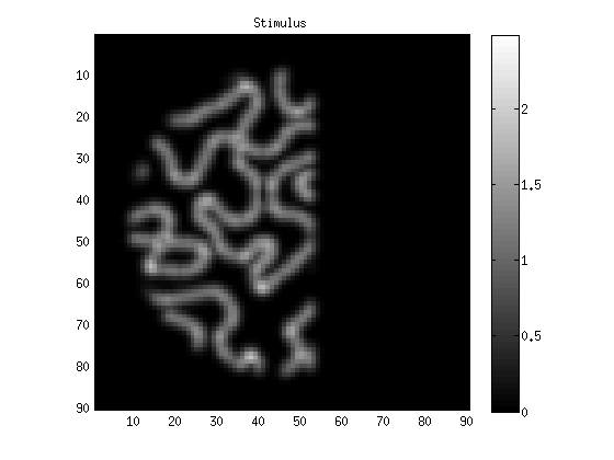
figure;
mx = max(abs(stimulus(:)));
imagesc(reshape(stimulus(12,:,1),[90 90]));
axis image tight;
caxis([0 mx]);
colormap(gray);
colorbar;
title('Stimulus');

% notice that the stimulus is now a "contrast image" where each value indicates
% the amount of local contrast at a particular location in the stimulus.

Prepare for model fitting

% to prepare for the call to fitnonlinearmodel.m, we have to define various
% input parameters.  this is what we will now do.

% define constants
res = 90;  % resolution of the pre-processed stimuli

% in this example script, we will be fitting only some of the parameters of the
% SOC model.  the other parameters have already been fixed (see above).
%
% the parameters that we will be fitting are [R C S G N C] where
%   R is the row index of the center of the 2D Gaussian
%   C is the column index of the center of the 2D Gaussian
%   S is the standard deviation of the 2D Gaussian
%   G is a gain parameter
%   N is the exponent of the power-law nonlinearity
%   C is a parameter that controls the strength of second-order contrast

% define initial seeds for model parameters.  to help avoid the problem of
% local minima, we will start at several different initial seeds (corresponding to
% different combinations of N and C), and we will choose the model that
% achieves the best fit to the data.
Ns = [.05 .1 .3 .5];
Cs = [.4 .7 .9 .95];
seeds = [];
for p=1:length(Ns)
  for q=1:length(Cs)
    seeds = cat(1,seeds,[(1+res)/2 (1+res)/2 res/4*sqrt(0.5) 10 Ns(p) Cs(q)]);
  end
end

% define bounds for the model parameters
bounds = [1-res+1 1-res+1 0   -Inf 0   0;
          2*res-1 2*res-1 Inf  Inf Inf 1];

% define a version of bounds where we insert NaNs in the first row
% in the spots corresponding to the N and C parameters.  this
% indicates to fix these parameters and not optimize them.
boundsFIX = bounds;
boundsFIX(1,5:6) = NaN;

% issue a dummy call to makegaussian2d.m to pre-compute xx and yy.
% these variables are re-used to achieve faster computation.
[d,xx,yy] = makegaussian2d(res,2,2,2,2);

% define a helper function that we will use for the SOC model.
% this function accepts stimuli (dd, a matrix of size A x 90*90),
% weights (wts, a vector of size 90*90 x 1), and a parameter
% (c, a scalar) and outputs a measure of variance (as a vector
% of size A x 1).  intuitively, this function computes
% a weighted average, subtracts that off, squares, and
% computes a weighted sum.
socfun = @(dd,wts,c) bsxfun(@minus,dd,c*(dd*wts)).^2 * wts;

% define another helper function.  given a set of parameters,
% this function outputs a 2D Gaussian (as a vector of size 90*90 x 1)
gaufun = @(pp) vflatten(makegaussian2d(res,pp(1),pp(2),pp(3),pp(3),xx,yy,0,0)/(2*pi*pp(3)^2));

% we will now define a function that implements the SOC model.  this function
% accepts a set of parameters (pp, a vector of size 1 x 6) and a set of stimuli
% (dd, a matrix of size A x 90*90) and outputs the predicted response to those
% stimuli (as a vector of size A x 1).
modelfun = @(pp,dd) pp(4)*(socfun(dd,gaufun(pp),restrictrange(pp(6),0,1)).^pp(5));

% notice that in the above function, we use restrictrange to force C to be
% between 0 and 1.  this is necessary because even though we defined bounds
% for the parameters (see above), we will be using the Levenberg-Marquardt
% optimization algorithm, which does not respect parameter bounds.

% we are ready to define the final model specification.  in the following,
% we specify a stepwise fitting scheme.  in the first fit (the first row),
% we start at the seed and optimize all parameters except the N and C parameters.
% in the second fit (the second row), we start at the parameters estimated in
% the first fit and optimize all parameters.  the reason that the first entry
% is [] is that we will be using a mechanism that evaluates multiple initial
% seeds, and in that case the first entry here is ignored.
model = {{[]         boundsFIX   modelfun} ...
         {@(ss) ss   bounds      @(ss) modelfun}};

% define optimization options (these are added on top of
% the default options used in fitnonlinearmodel.m)
optimoptions = {'Algorithm' 'levenberg-marquardt' 'Display' 'off'};

% define the resampling scheme to use.  here, we use 0, which
% means to just fit the data (no cross-validation nor bootstrapping).
resampling = 0;

% define the metric that we will use to quantify goodness-of-fit.
metric = @(a,b) calccod(a,b,[],[],0);

% specify the index of the voxel to fit
ix = 204;

% finally, construct the options struct that will be passed to fitnonlinearmodel.m
opt = struct( ...
  'stimulus',     stimulus, ...
  'data',         betamn(ix,1:99)', ...
  'model',        {model}, ...
  'seed',         seeds, ...
  'optimoptions', {optimoptions}, ...
  'resampling',   resampling, ...
  'metric',       metric);

% do a quick inspection of opt
opt

opt = 

        stimulus: [99x8100x9 single]
            data: [99x1 double]
           model: {{1x3 cell}  {1x3 cell}}
            seed: [16x6 double]
    optimoptions: {'Algorithm'  'levenberg-marquardt'  'Display'  'off'}
      resampling: 0
          metric: @(a,b)calccod(a,b,[],[],0)

Fit the model

results = fitnonlinearmodel(opt);

*** fitnonlinearmodel: started at 28-Aug-2013 15:10:47. ***
*** fitnonlinearmodel: outputdir = , chunksize = 1, chunknum = 1
*** fitnonlinearmodel: processing voxel 1 (1 of 1). ***
  starting resampling case 1 of 1.
    trying seed 1 of 16.
      for model 1 of 2, the seed is [45.500 45.500 15.910 10.000 0.050 0.400 ].
      the estimated parameters are [55.763 60.759 1.075 6.241 0.050 0.400 ].
      for model 2 of 2, the seed is [55.763 60.759 1.075 6.241 0.050 0.400 ].
      the estimated parameters are [53.152 57.367 1.289 6.004 0.105 0.193 ].
    trying seed 2 of 16.
      for model 1 of 2, the seed is [45.500 45.500 15.910 10.000 0.050 0.700 ].
      the estimated parameters are [56.422 61.855 1.082 6.701 0.050 0.700 ].
      for model 2 of 2, the seed is [56.422 61.855 1.082 6.701 0.050 0.700 ].
      the estimated parameters are [53.749 59.030 1.234 7.208 0.123 0.715 ].
    trying seed 3 of 16.
      for model 1 of 2, the seed is [45.500 45.500 15.910 10.000 0.050 0.900 ].
      the estimated parameters are [56.545 61.231 1.304 6.544 0.050 0.900 ].
      for model 2 of 2, the seed is [56.545 61.231 1.304 6.544 0.050 0.900 ].
      the estimated parameters are [54.061 57.207 1.392 9.173 0.168 0.862 ].
    trying seed 4 of 16.
      for model 1 of 2, the seed is [45.500 45.500 15.910 10.000 0.050 0.950 ].
      the estimated parameters are [80.008 87.283 4.416 9.646 0.050 0.950 ].
      for model 2 of 2, the seed is [80.008 87.283 4.416 9.646 0.050 0.950 ].
      the estimated parameters are [70.499 81.121 5.406 7.895 0.106 0.689 ].
    trying seed 5 of 16.
      for model 1 of 2, the seed is [45.500 45.500 15.910 10.000 0.100 0.400 ].
      the estimated parameters are [54.139 60.840 1.681 6.625 0.100 0.400 ].
      for model 2 of 2, the seed is [54.139 60.840 1.681 6.625 0.100 0.400 ].
      the estimated parameters are [54.105 61.161 1.635 7.906 0.147 0.669 ].
    trying seed 6 of 16.
      for model 1 of 2, the seed is [45.500 45.500 15.910 10.000 0.100 0.700 ].
      the estimated parameters are [73.527 76.438 5.492 7.006 0.100 0.700 ].
      for model 2 of 2, the seed is [73.527 76.438 5.492 7.006 0.100 0.700 ].
      the estimated parameters are [73.527 76.438 5.492 7.006 0.100 0.700 ].
    trying seed 7 of 16.
      for model 1 of 2, the seed is [45.500 45.500 15.910 10.000 0.100 0.900 ].
      the estimated parameters are [61.395 66.003 2.998 7.447 0.100 0.900 ].
      for model 2 of 2, the seed is [61.395 66.003 2.998 7.447 0.100 0.900 ].
      the estimated parameters are [56.215 61.618 2.810 9.365 0.201 0.849 ].
    trying seed 8 of 16.
      for model 1 of 2, the seed is [45.500 45.500 15.910 10.000 0.100 0.950 ].
      the estimated parameters are [60.598 70.078 3.031 7.260 0.100 0.950 ].
      for model 2 of 2, the seed is [60.598 70.078 3.031 7.260 0.100 0.950 ].
      the estimated parameters are [56.299 61.868 2.775 8.887 0.199 0.784 ].
    trying seed 9 of 16.
      for model 1 of 2, the seed is [45.500 45.500 15.910 10.000 0.300 0.400 ].
      the estimated parameters are [58.553 65.802 4.827 7.799 0.300 0.400 ].
      for model 2 of 2, the seed is [58.553 65.802 4.827 7.799 0.300 0.400 ].
      the estimated parameters are [57.411 63.666 3.724 9.288 0.222 0.816 ].
    trying seed 10 of 16.
      for model 1 of 2, the seed is [45.500 45.500 15.910 10.000 0.300 0.700 ].
      the estimated parameters are [60.161 62.370 5.223 9.567 0.300 0.700 ].
      for model 2 of 2, the seed is [60.161 62.370 5.223 9.567 0.300 0.700 ].
      the estimated parameters are [56.237 62.297 3.107 9.806 0.229 0.834 ].
    trying seed 11 of 16.
      for model 1 of 2, the seed is [45.500 45.500 15.910 10.000 0.300 0.900 ].
      the estimated parameters are [59.754 66.511 5.399 10.820 0.300 0.900 ].
      for model 2 of 2, the seed is [59.754 66.511 5.399 10.820 0.300 0.900 ].
      the estimated parameters are [60.425 66.786 5.401 10.466 0.284 0.904 ].
    trying seed 12 of 16.
      for model 1 of 2, the seed is [45.500 45.500 15.910 10.000 0.300 0.950 ].
      the estimated parameters are [60.237 66.872 5.742 10.710 0.300 0.950 ].
      for model 2 of 2, the seed is [60.237 66.872 5.742 10.710 0.300 0.950 ].
      the estimated parameters are [60.237 66.872 5.742 10.710 0.300 0.950 ].
    trying seed 13 of 16.
      for model 1 of 2, the seed is [45.500 45.500 15.910 10.000 0.500 0.400 ].
      the estimated parameters are [53.193 65.116 12.302 7.352 0.500 0.400 ].
      for model 2 of 2, the seed is [53.193 65.116 12.302 7.352 0.500 0.400 ].
      the estimated parameters are [56.460 61.532 3.112 10.141 0.241 0.840 ].
    trying seed 14 of 16.
      for model 1 of 2, the seed is [45.500 45.500 15.910 10.000 0.500 0.700 ].
      the estimated parameters are [56.418 59.072 11.814 10.450 0.500 0.700 ].
      for model 2 of 2, the seed is [56.418 59.072 11.814 10.450 0.500 0.700 ].
      the estimated parameters are [60.413 67.954 4.552 9.426 0.210 1.082 ].
    trying seed 15 of 16.
      for model 1 of 2, the seed is [45.500 45.500 15.910 10.000 0.500 0.900 ].
      the estimated parameters are [58.765 64.525 6.499 15.015 0.500 0.900 ].
      for model 2 of 2, the seed is [58.765 64.525 6.499 15.015 0.500 0.900 ].
      the estimated parameters are [59.142 64.366 6.525 14.717 0.484 0.894 ].
    trying seed 16 of 16.
      for model 1 of 2, the seed is [45.500 45.500 15.910 10.000 0.500 0.950 ].
      the estimated parameters are [59.894 64.637 6.581 14.968 0.500 0.950 ].
      for model 2 of 2, the seed is [59.894 64.637 6.581 14.968 0.500 0.950 ].
      the estimated parameters are [60.064 65.534 6.221 14.066 0.442 1.020 ].
    seed 3 was best. final estimated parameters are [54.061 57.207 1.392 9.173 0.168 0.862 ].
*** fitnonlinearmodel: voxel 1 (1 of 1) took 136.4 seconds. ***
*** fitnonlinearmodel: ended at 28-Aug-2013 15:13:04 (2.3 minutes). ***

Inspect the results

% these are the final parameter estimates
results.params

ans =

  Columns 1 through 3

          54.0608173443624           57.207123537548          1.39186915322788

  Columns 4 through 6

          9.17342790703929         0.168132144998856         0.861591769911232

% this is the R^2 between the model fit and the data
results.trainperformance

ans =

          95.1740363925398

% visualize the data and the model fit
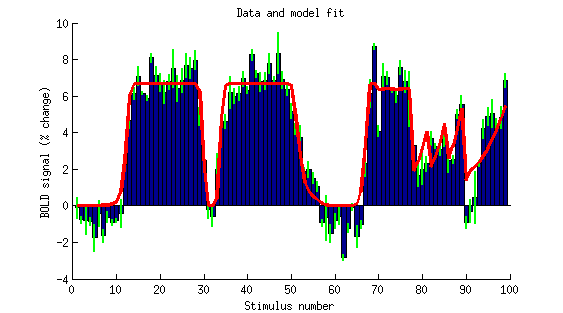
figure; setfigurepos([100 100 450 250]); hold on;
bar(betamn(ix,1:99),1);
errorbar2(1:99,betamn(ix,1:99),betase(ix,1:99),'v','g-','LineWidth',2);
modelfit = [];
for p=1:9
  modelfit(:,p) = modelfun(results.params,stimulus(:,:,p));
end
plot(1:99,mean(modelfit,2),'r-','LineWidth',3);
ax = axis;
axis([0 100 ax(3:4)]);
xlabel('Stimulus number');
ylabel('BOLD signal (% change)');
title('Data and model fit');

Published with MATLAB® R2012b