Example script illustrating the third dataset

Contents

Load in the third dataset

% load in the data
load('dataset03.mat');

% check the workspace
whos

  Name              Size                   Bytes  Class      Attributes

  betamn         1323x156                1651104  double               
  betas          1323x156x30            49533120  double               
  betase         1323x156                1651104  double               
  glmr2          1323x1                    10584  double               
  hrfmn          1323x38                  402192  double               
  hrfs           1323x38x30             12065760  double               
  hrfse          1323x38                  402192  double               
  meanvol          64x64x22               720896  double               
  roi            1323x1                    10584  double               
  roilabels         1x12                    1408  cell                 
  tr                1x1                        8  double               
  vxs            1323x1                    10584  double               
  vxsselect      1323x3                     3969  logical              

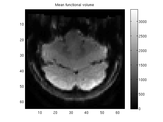
Inspect the data at a gross level

% look at the mean functional volume (slice #11)
figure;
imagesc(meanvol(:,:,11));
axis equal tight;
colorbar;
title('Mean functional volume');

% some of the voxels have positive cross-validation accuracy (R^2)
% when fit with the GLM model. these are the voxels that we use
% for further analysis. let's visualize R^2 values for these voxels.
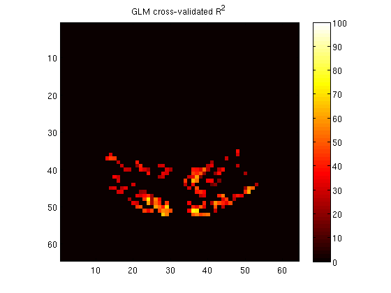
vol = zeros(size(meanvol));
vol(vxs) = glmr2;
figure;
imagesc(vol(:,:,11),[0 100]);
colormap(hot);
axis equal tight;
colorbar;
title('GLM cross-validated R^2');

% inspect the ROI assignments.
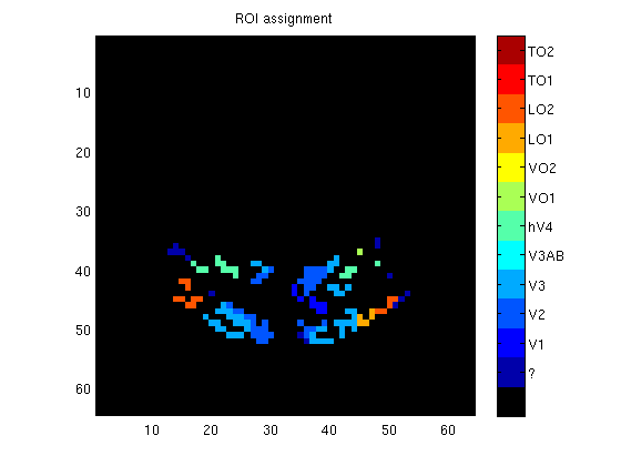
vol = zeros(size(meanvol));
vol(vxs) = roi;
figure;
imagesc(vol(:,:,11),[0-.5 12+.5]);
colormap([0 0 0; jet(12)]);
axis equal tight;
cb = colorbar;
set(cb,'YTick',1:12,'YTickLabel',roilabels);
title('ROI assignment');

Inspect the estimated HRF and beta weights for one voxel

% let's pick a voxel
goodvoxels = find(glmr2 > 70);
ii = goodvoxels(1);

% report some information
fprintf('The chosen voxel is the %dth voxel of the %d voxels contained in the data file.\n',ii,length(vxs));
fprintf('The absolute index of this voxel is %d.\n',vxs(ii));
fprintf('The ROI assignment is %s.\n',roilabels{roi(ii)});
fprintf('The GLM R^2 for this voxel is %.1f.\n',glmr2(ii));

The chosen voxel is the 203th voxel of the 1323 voxels contained in the data file.
The absolute index of this voxel is 26926.
The ROI assignment is V1.
The GLM R^2 for this voxel is 72.2.

% plot the HRF
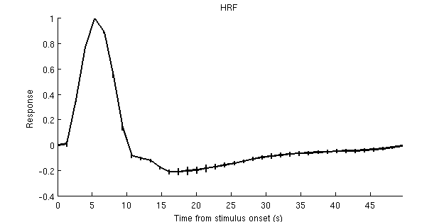
figure; hold on;
set(gcf,'Units','points','Position',[100 100 500 250]);
xx = 0:tr:tr*(size(hrfmn,2)-1);  % time points at which the HRF is sampled
yy = hrfmn(ii,:);
ee = hrfse(ii,:);
plot(xx,yy,'k-','LineWidth',2);
for p=1:length(yy)
  plot([xx(p) xx(p)],[yy(p)-ee(p) yy(p)+ee(p)],'k-','LineWidth',2);
end
ax = axis; axis([xx(1) xx(end) ax(3:4)]);
xlabel('Time from stimulus onset (s)');
ylabel('Response');
title('HRF');

% plot the beta weights
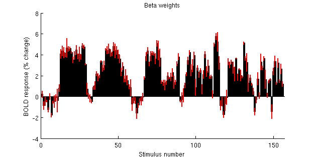
figure; hold on;
set(gcf,'Units','points','Position',[100 100 500 250]);
n = size(betas,2);  % number of stimuli
yy = betamn(ii,:);
ee = betase(ii,:);
bar(1:n,yy,1);
for p=1:n
  plot([p p],[yy(p)-ee(p) yy(p)+ee(p)],'r-','LineWidth',2);
end
ax = axis; axis([0 n+1 ax(3:4)]);
xlabel('Stimulus number');
ylabel('BOLD response (% change)');
title('Beta weights');

Published with MATLAB® 7.9