 |
 |
 |
 |
|
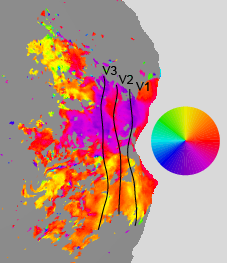
Angle
|
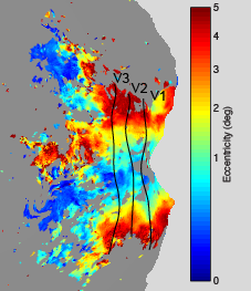
Eccentricity
|
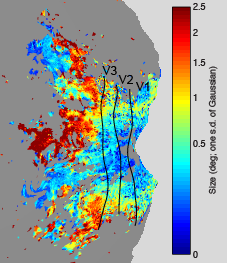
Size
|
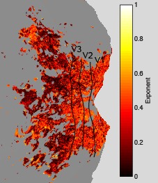
Exponent
|
| analyzePRF: stimuli
and code for pRF analysis Kendrick Kay Questions, comments? E-mail Kendrick |
The population receptive field (pRF) technique described in Dumoulin and Wandell (2008) provides a means for estimating the aggregate receptive field of populations of neurons as measured with fMRI. On this web site, we provide:
Because the code is general, it is not necessary to use the stimuli provided here; the code can be used in a standalone fashion to analyze a variety of data.
The specific pRF model that we implement is the Compressive Spatial Summation (CSS) model, which is similar to the original model (2D isotropic Gaussian), except that a static power-law nonlinearity is added after summation across the visual field. The nonlinearity is typically compressive, hence the name of the model. The CSS model is described in the following paper:
If you use analyzePRF, consider citing the above paper, as well as potentially the original Dumoulin and Wandell (2008) paper.
Regarding the stimuli, the stimuli are described and used in the HCP 7T Retinotopy Dataset paper.
Terms of use: The content provided by this web site is licensed under a Creative Commons Attribution 3.0 Unported License. You are free to share and adapt the content as you please, under the condition that you cite the appropriate manuscripts.
Acknowledgements: Thanks to An Vu for 7T data collection and advice on stimulus design.
The following maps were obtained from a pRF experiment (3T, 2.5-mm resolution, 2-s TR, 20 minutes of data, 10° field of view, simple fixation task). The maps are flatmaps of the left hemisphere, and they have been thresholded based on variance explained.
|
|
|
|
|
|
Angle
|
Eccentricity
|
Size
|
Exponent
|
Contents of 'stimuli.mat':
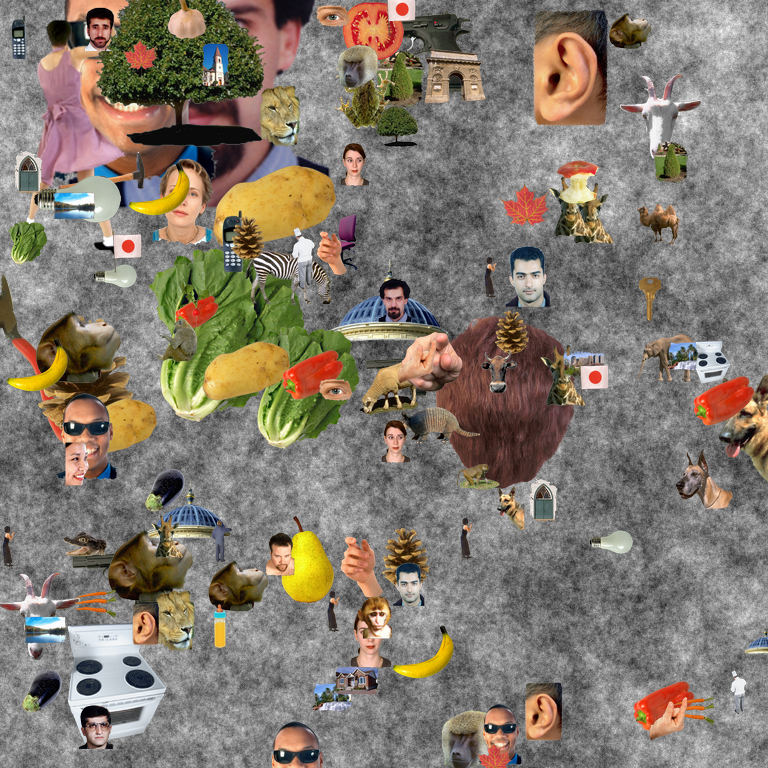
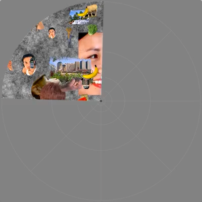
'patterns' is 768 x 768 x 3 x 100 (uint8 format) with RGB images at a resolution of 768 pixels x 768 pixels. There are 100 different images, corresponding to different random draws of the pattern. The pattern consists of color objects at multiple spatial scales placed on a pink-noise background. The pattern is designed to drive both low-level and high-level visual areas. The following is a sample of one of the images (click for the full-sized version):
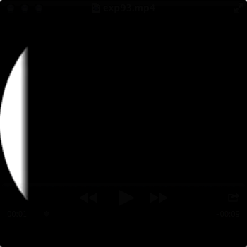
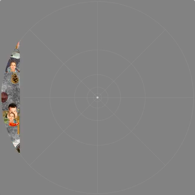
'masks' is 768 x 768 x 2580 (uint8 format) with masks that are to be applied to the patterns. There are 2580 different masks. The values in the masks range from 0 to 255 (0 means do not pass the pattern; 255 means fully pass the pattern). The following is a thumbnail of one of the masks:
'multibarindices' is a 1 x 4500 vector with mask indices. The indices in this vector indicate which masks to present and when to present them. 0 is used to indicate that no mask is to be presented (i.e. rest periods). This "multibar" stimulus consists of bars that sweep in multiple different directions. The bar sweeps occur in 32-second chunks, each of which consists of a 28-second sweep followed by a 4-second rest. The intended frame rate is 15 Hz; thus, the total run duration is 4500/15 = 300 seconds = 5 minutes. The overall temporal structure is [16-second rest, L-R, D-U, R-L, U-D, 12-second rest, LL-UR, LR-UL, UR-LL, UL-LR, 16-second rest] = [16+32*4+12+32*4+16=300]. The following is a movie that illustrates the mask design (click for the movie):
'wedgeringindices' is a 1 x 4500 vector with mask indices, similar to 'multibarindices'. This "wedgering" stimulus consists of rotating wedges and expanding and contracting rings. The wedges revolve in 32 seconds; the rings sweep for 28 seconds and are followed by 4 seconds of rest. The total run duration is 4500/15 = 300 seconds = 5 minutes. The overall temporal structure is [22-second rest, CCW, CCW, expand, expand, CW, CW, contract, contract, 22-second rest] = [22+32*8+22=300]. The following is a movie that illustrates the mask design (click for the movie):
Sample stimulus movies:
The final stimuli are generated by applying the masks to the patterns. The following is a short movie clip showing what the actual multibar stimulus looks like (note that the fixation dot and fixation grid are extra components that are included in our particular presentation environment):
The following is a short movie clip showing what the actual wedgering stimulus looks like:
You can adapt the stimuli provided above in your
own presentation setup. Or, you can use the code provided here.
The presentation code is in MATLAB and relies on Psychtoolbox. The
stimuli are constructed at a size of 768 x 768 and are intended
for a 60-Hz display. Thus, a display resolution of 1024 x 768 @ 60
Hz is ideal.
Installation steps:
Note that the runretinotopy* files are located in knkutils/pt/.
analyzePRF is a MATLAB toolbox that estimates pRFs from fMRI data.
Download code from github
After downloading and unzipping the files, launch MATLAB and
change to the directory containing the files. You can then run the
example scripts by typing "example1", "example2", etc. More
information on the example scripts is provided below.
Download
example dataset (4 MB)
This dataset is required to run the example scripts. Place the
dataset inside the code directory. Alternatively, the example
scripts will automatically download the dataset.
Download
example stimulus pre-processing script
This is an example script that shows how one might prepare the raw
stimulus masks for purposes of data analysis.
Browse code in HTML (code tagged version 1.1)
The basics. In a nutshell, the code can be thought of as a black box that takes fMRI data and outputs pRF parameter estimates. The code is general; it does not require phase-encoded data but can also be used to analyze event-related and multifocal data. The code assumes that the fMRI data have been pre-processed. We recommend that at a minimum, slice time correction and motion correction should be performed and the first few volumes of each run should be discarded (if not already performed by the scanner) to allow magnetization to reach steady-state. Polynomial regressors are included in the pRF model, so the data do not need to be detrended or high-pass filtered.
Code execution. The most basic call to the code is:
results = analyzePRF(stimulus,data,tr,struct('seedmode',2));
where 'stimulus' specifies the masks used in the experiment, 'data' specifies the fMRI time-series data, 'tr' specifies the TR in seconds, and 'seedmode' specifies the strategy for the initial seed. Details on the inputs and outputs of analyzePRF.m are provided in the code documentation.
Example scripts. The following are HTML pages automatically produced by the MATLAB publish command:
GLMdenoise. analyzePRF includes the capability to use GLMdenoise to denoise the pRF estimates. For simplicity, the use of GLMdenoise is off by default.
Cluster computing. analyzePRF includes some skeleton code for executing pRF analyses in a cluster-computing environment. However, cluster implementations must be tailored on a case-by-case basis, so the cluster feature will not work "out of the box".
Speed issues. Fitting
pRF models is computationally intensive. To reduce execution time,
one could use fewer initial seeds (at the risk of obtaining poorer
fits (i.e. getting stuck in a local minimum)) or select a smaller
set of voxels to analyze. The 'seedmode'==2 strategy uses just one
initial seed (chosen from a large library of seeds).
HRF issues. The default
strategy in analyzePRF is to assume a canonical hemodynamic
response function (HRF). This is a potential source of inaccuracy.
However, with an appropriately balanced design (e.g. both CCW and
CW wedges) and a simple pRF model (e.g. a model that has only
excitatory regions), the risk is likely minimal.