Example 4: Use GLMdenoise, allowing voxel-specific HRFs

Contents

Download dataset (if necessary) and add GLMdenoise to the MATLAB path

setup;

Load in the data

% Load in the data
load('exampledataset.mat');

% Check the workspace
whos

  Name         Size                Bytes  Class     Attributes

  data         1x10            173671520  cell                
  design       1x10                 9600  cell                
  stimdur      1x1                     8  double              
  tr           1x1                     8  double              

Outline the strategy

% Fitting the finite impulse response (FIR) model is at one end of the spectrum of
% allowing flexibility in estimated hemodynamic response functions (HRFs).  However,
% there is a real potential for the FIR model to overfit, especially when there is a
% large number of conditions.  A less aggressive strategy is to allow each voxel
% (or ROI) to have its own flexible HRF but enforce the constraint that the same HRF
% applies to different conditions (thus, the conditions differ only with respect
% to their associated beta weights).
%
% The default behavior of GLMdenoisedata is to optimize the HRF to best fit the
% top 50 voxels in the dataset.  Suppose, however, that we want to instead
% optimize the HRF on a voxel-by-voxel basis.  One challenge in this approach
% is computational time, as an iterative fitting procedure must be performed
% for each voxel in the dataset.  The other challenge is how this can co-exist
% with the denoising technique implemented in GLMdenoise.
%
% Our strategy is as follows.  First, we will make an initial call to GLMdenoise,
% assuming a canonical HRF (which is computed based on the stimulus duration and
% the TR).  The point of this initial call is to learn the noise regressors
% (and the specific number of noise regressors) that result in good cross-validation
% performance.  Then, we will re-analyze the data voxel-by-voxel, including the noise
% regressors learned in the first step and tailoring the HRF on a voxel-by-voxel basis.

Step 1: Initial call to GLMdenoise to learn the noise regressors

% Compute a canonical HRF.
hrf = getcanonicalhrf(stimdur,tr)';

% Make the initial call to GLMdenoise.  We indicate that the canonical HRF is to be
% assumed.  We also turn off bootstrapping as it is unnecessary here.
results = GLMdenoisedata(design,data,stimdur,tr, ...
            'assume',hrf,struct('numboots',0), ...
            'example4figures');

% Extract the noise regressors based on the results.  Note that results.pcnum is
% the number of noise regressors that was selected by GLMdenoisedata.m.
noisereg = cellfun(@(x) x(:,1:results.pcnum),results.pcregressors,'UniformOutput',0);

% Inspect the dimensionality of the noise regressors.
noisereg

*** GLMdenoisedata: generating sanity-check figures. ***
*** GLMdenoisedata: performing cross-validation to determine R^2 values. ***
cross-validating model..........done.
computing model fits...done.
computing R^2...done.
computing SNR...done.
*** GLMdenoisedata: determining noise pool. ***
*** GLMdenoisedata: calculating noise regressors. ***
*** GLMdenoisedata: performing cross-validation with 1 PCs. ***
cross-validating model..........done.
computing model fits...done.
computing R^2...done.
computing SNR...done.
*** GLMdenoisedata: performing cross-validation with 2 PCs. ***
cross-validating model..........done.
computing model fits...done.
computing R^2...done.
computing SNR...done.
*** GLMdenoisedata: performing cross-validation with 3 PCs. ***
cross-validating model..........done.
computing model fits...done.
computing R^2...done.
computing SNR...done.
*** GLMdenoisedata: performing cross-validation with 4 PCs. ***
cross-validating model..........done.
computing model fits...done.
computing R^2...done.
computing SNR...done.
*** GLMdenoisedata: performing cross-validation with 5 PCs. ***
cross-validating model..........done.
computing model fits...done.
computing R^2...done.
computing SNR...done.
*** GLMdenoisedata: performing cross-validation with 6 PCs. ***
cross-validating model..........done.
computing model fits...done.
computing R^2...done.
computing SNR...done.
*** GLMdenoisedata: performing cross-validation with 7 PCs. ***
cross-validating model..........done.
computing model fits...done.
computing R^2...done.
computing SNR...done.
*** GLMdenoisedata: performing cross-validation with 8 PCs. ***
cross-validating model..........done.
computing model fits...done.
computing R^2...done.
computing SNR...done.
*** GLMdenoisedata: performing cross-validation with 9 PCs. ***
cross-validating model..........done.
computing model fits...done.
computing R^2...done.
computing SNR...done.
*** GLMdenoisedata: performing cross-validation with 10 PCs. ***
cross-validating model..........done.
computing model fits...done.
computing R^2...done.
computing SNR...done.
*** GLMdenoisedata: performing cross-validation with 11 PCs. ***
cross-validating model..........done.
computing model fits...done.
computing R^2...done.
computing SNR...done.
*** GLMdenoisedata: performing cross-validation with 12 PCs. ***
cross-validating model..........done.
computing model fits...done.
computing R^2...done.
computing SNR...done.
*** GLMdenoisedata: performing cross-validation with 13 PCs. ***
cross-validating model..........done.
computing model fits...done.
computing R^2...done.
computing SNR...done.
*** GLMdenoisedata: performing cross-validation with 14 PCs. ***
cross-validating model..........done.
computing model fits...done.
computing R^2...done.
computing SNR...done.
*** GLMdenoisedata: performing cross-validation with 15 PCs. ***
cross-validating model..........done.
computing model fits...done.
computing R^2...done.
computing SNR...done.
*** GLMdenoisedata: performing cross-validation with 16 PCs. ***
cross-validating model..........done.
computing model fits...done.
computing R^2...done.
computing SNR...done.
*** GLMdenoisedata: performing cross-validation with 17 PCs. ***
cross-validating model..........done.
computing model fits...done.
computing R^2...done.
computing SNR...done.
*** GLMdenoisedata: performing cross-validation with 18 PCs. ***
cross-validating model..........done.
computing model fits...done.
computing R^2...done.
computing SNR...done.
*** GLMdenoisedata: performing cross-validation with 19 PCs. ***
cross-validating model..........done.
computing model fits...done.
computing R^2...done.
computing SNR...done.
*** GLMdenoisedata: performing cross-validation with 20 PCs. ***
cross-validating model..........done.
computing model fits...done.
computing R^2...done.
computing SNR...done.
*** GLMdenoisedata: selected number of PCs is 6. ***
*** GLMdenoisedata: fitting final model (no denoising, for comparison purposes). ***
fitting model...done.
preparing output...done.
computing model fits...done.
computing R^2...done.
computing SNR...done.
*** GLMdenoisedata: fitting final model (with denoising). ***
fitting model...done.
preparing output...done.
computing model fits...done.
computing R^2...done.
computing SNR...done.
*** GLMdenoisedata: calculating denoised data and PC weights. ***
*** GLMdenoisedata: converting to percent BOLD change. ***
*** GLMdenoisedata: generating figures. ***

noisereg = 

  Columns 1 through 4

    [265x6 single]    [265x6 single]    [265x6 single]    [265x6 single]

  Columns 5 through 8

    [265x6 single]    [265x6 single]    [265x6 single]    [265x6 single]

  Columns 9 through 10

    [265x6 single]    [265x6 single]

Step 2: Re-analyze the data, tailoring the HRF voxel-by-voxel

% Define some useful constants.
xyzsize = [64 64 4];  % the XYZ dimensions of the dataset
numcond = 35;         % the number of conditions in this dataset

% Define an options struct.  This specifies (1) that the noise regressors determined
% above will serve as extra regressors in the GLM, (2) that the HRF estimated
% from the data should always be used (even if it is very unlike the initial seed),
% and (3) that we want to suppress text output (since many voxels will be analyzed
% in a loop).
opt = struct('extraregressors',{noisereg},'hrfthresh',-Inf,'suppressoutput',1);

% Initialize the results.
hrfs = zeros([xyzsize length(hrf)],'single');
betas = zeros([xyzsize numcond],'single');
R2 = zeros([xyzsize],'single');

% Loop over voxels.  Note: The following loop may take a long time to execute.
% This loop can be speeded up using parfor or cluster-computing solutions, but
% here we use a simple for-loop for the purpose of simplicity.
cache = [];
for xx=1:xyzsize(1)
  fprintf('#');
  for yy=1:xyzsize(2)
    fprintf('.');
    for zz=1:xyzsize(3)

      % Extract the time-series data for one voxel.
      data0 = cellfun(@(x) flatten(x(xx,yy,zz,:)),data,'UniformOutput',0);

      % Analyze the time-series, specifying that we want to optimize the HRF.
      % We use the canonical HRF as the initial seed for the HRF.
      [results0,cache] = GLMestimatemodel(design,data0,stimdur,tr, ...
                           'optimize',hrf,0,opt,cache);

      % Record the results.
      hrfs(xx,yy,zz,:) = results0.modelmd{1};
      betas(xx,yy,zz,:) = results0.modelmd{2};
      R2(xx,yy,zz) = results0.R2;

    end
  end
end

#................................................................#................................................................#................................................................#................................................................#................................................................#................................................................#................................................................#................................................................#................................................................#................................................................#................................................................#................................................................#................................................................#................................................................#................................................................#................................................................#................................................................#................................................................#................................................................#................................................................#................................................................#................................................................#................................................................#................................................................#................................................................#................................................................#................................................................#................................................................#................................................................#................................................................#................................................................#................................................................#................................................................#................................................................#................................................................#................................................................#................................................................#................................................................#................................................................#................................................................#................................................................#................................................................#................................................................#................................................................#................................................................#................................................................#................................................................#................................................................#................................................................#................................................................#................................................................#................................................................#................................................................#................................................................#................................................................#................................................................#................................................................#................................................................#................................................................#................................................................#................................................................#................................................................#................................................................#................................................................

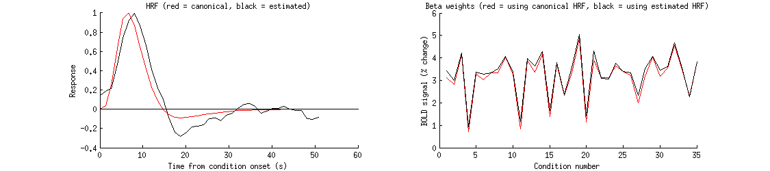
Inspect the results

% Here we inspect the results for an example voxel.  Notice that the estimated HRF
% is a bit delayed with respect to the canonical HRF.  The beta weights across
% the two cases, however, are pretty similar.
xx = 53; yy = 27; zz = 1;
figure;
set(gcf,'Units','points','Position',[100 100 900 200]);
subplot(1,2,1); hold on;
plot(0:tr:(length(hrf)-1)*tr,hrf,'r-');
plot(0:tr:(length(hrf)-1)*tr,flatten(hrfs(xx,yy,zz,:)),'k-');
straightline(0,'h','k-');
xlabel('Time from condition onset (s)');
ylabel('Response');
title('HRF (red = canonical, black = estimated)');
subplot(1,2,2); hold on;
plot(flatten(results.modelmd{2}(xx,yy,zz,:)),'r-');
plot(flatten(betas(xx,yy,zz,:)),'k-');
straightline(0,'h','k-');
xlabel('Condition number');
ylabel('BOLD signal (% change)');
title('Beta weights (red = using canonical HRF, black = using estimated HRF)');

Published with MATLAB® R2012b