Example 1: Run GLMdenoise on an example dataset

Contents

Download dataset (if necessary) and add GLMdenoise to the MATLAB path

setup;

Load in the data

% Load in the data
load('exampledataset.mat');

% Check the workspace
whos

  Name         Size                Bytes  Class     Attributes

  data         1x10            173671520  cell                
  design       1x10                 9600  cell                
  stimdur      1x1                     8  double              
  tr           1x1                     8  double              

Inspect the data

% Look at the design matrix for the first run.  Notice that there are
% 35 conditions and each condition is presented once during the run.
figure;
set(gcf,'Units','points','Position',[100 100 350 500]);
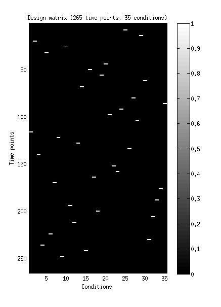
imagesc(design{1});
colormap(gray);
colorbar;
xlabel('Conditions');
ylabel('Time points');
title(sprintf('Design matrix (%d time points, %d conditions)',size(design{1},1),size(design{1},2)));

% Look at the first volume of the first run.  We split the volume along
% the third dimension (the slice dimension) and show slices starting at the
% upper-left, proceeding downwards, and then from left to right.
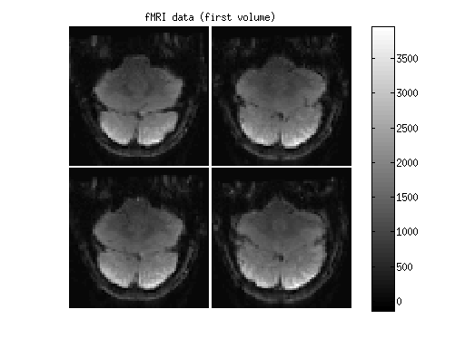
figure;
imagesc(makeimagestack(data{1}(:,:,:,1)));
colormap(gray);
axis equal tight off;
colorbar;
title('fMRI data (first volume)');

% Check various constants
fprintf('There are %d runs in total.\n',length(design));
fprintf('The dimensions of the data for the first run are %s.\n',mat2str(size(data{1})));
fprintf('The stimulus duration is %.6f seconds.\n',stimdur);
fprintf('The sampling rate (TR) is %.6f seconds.\n',tr);

There are 10 runs in total.
The dimensions of the data for the first run are [64 64 4 265].
The stimulus duration is 3.000000 seconds.
The sampling rate (TR) is 1.337702 seconds.

Run GLMdenoise

% Call GLMdenoise using default parameters.  Outputs will be stored in
% 'results' and 'denoiseddata'.  Figures will be written to 'example1figures'
% in the current directory.
[results,denoiseddata] = GLMdenoisedata(design,data,stimdur,tr,[],[],[],'example1figures');

*** GLMdenoisedata: performing full fit to estimate global HRF. ***
fitting model...done.
preparing output...done.
computing model fits...done.
computing R^2...done.
computing SNR...done.
*** GLMdenoisedata: performing cross-validation to determine R^2 values. ***
cross-validating model..........done.
computing model fits...done.
computing R^2...done.
computing SNR...done.
*** GLMdenoisedata: determining noise pool. ***
*** GLMdenoisedata: calculating global noise regressors. ***
*** GLMdenoisedata: performing cross-validation with 1 PCs. ***
cross-validating model..........done.
computing model fits...done.
computing R^2...done.
computing SNR...done.
*** GLMdenoisedata: performing cross-validation with 2 PCs. ***
cross-validating model..........done.
computing model fits...done.
computing R^2...done.
computing SNR...done.
*** GLMdenoisedata: performing cross-validation with 3 PCs. ***
cross-validating model..........done.
computing model fits...done.
computing R^2...done.
computing SNR...done.
*** GLMdenoisedata: performing cross-validation with 4 PCs. ***
cross-validating model..........done.
computing model fits...done.
computing R^2...done.
computing SNR...done.
*** GLMdenoisedata: performing cross-validation with 5 PCs. ***
cross-validating model..........done.
computing model fits...done.
computing R^2...done.
computing SNR...done.
*** GLMdenoisedata: performing cross-validation with 6 PCs. ***
cross-validating model..........done.
computing model fits...done.
computing R^2...done.
computing SNR...done.
*** GLMdenoisedata: performing cross-validation with 7 PCs. ***
cross-validating model..........done.
computing model fits...done.
computing R^2...done.
computing SNR...done.
*** GLMdenoisedata: performing cross-validation with 8 PCs. ***
cross-validating model..........done.
computing model fits...done.
computing R^2...done.
computing SNR...done.
*** GLMdenoisedata: performing cross-validation with 9 PCs. ***
cross-validating model..........done.
computing model fits...done.
computing R^2...done.
computing SNR...done.
*** GLMdenoisedata: performing cross-validation with 10 PCs. ***
cross-validating model..........done.
computing model fits...done.
computing R^2...done.
computing SNR...done.
*** GLMdenoisedata: performing cross-validation with 11 PCs. ***
cross-validating model..........done.
computing model fits...done.
computing R^2...done.
computing SNR...done.
*** GLMdenoisedata: performing cross-validation with 12 PCs. ***
cross-validating model..........done.
computing model fits...done.
computing R^2...done.
computing SNR...done.
*** GLMdenoisedata: performing cross-validation with 13 PCs. ***
cross-validating model..........done.
computing model fits...done.
computing R^2...done.
computing SNR...done.
*** GLMdenoisedata: performing cross-validation with 14 PCs. ***
cross-validating model..........done.
computing model fits...done.
computing R^2...done.
computing SNR...done.
*** GLMdenoisedata: performing cross-validation with 15 PCs. ***
cross-validating model..........done.
computing model fits...done.
computing R^2...done.
computing SNR...done.
*** GLMdenoisedata: performing cross-validation with 16 PCs. ***
cross-validating model..........done.
computing model fits...done.
computing R^2...done.
computing SNR...done.
*** GLMdenoisedata: performing cross-validation with 17 PCs. ***
cross-validating model..........done.
computing model fits...done.
computing R^2...done.
computing SNR...done.
*** GLMdenoisedata: performing cross-validation with 18 PCs. ***
cross-validating model..........done.
computing model fits...done.
computing R^2...done.
computing SNR...done.
*** GLMdenoisedata: performing cross-validation with 19 PCs. ***
cross-validating model..........done.
computing model fits...done.
computing R^2...done.
computing SNR...done.
*** GLMdenoisedata: performing cross-validation with 20 PCs. ***
cross-validating model..........done.
computing model fits...done.
computing R^2...done.
computing SNR...done.
*** GLMdenoisedata: selected number of PCs is 6. ***
*** GLMdenoisedata: fitting final model (no denoising, for comparison purposes). ***
bootstrapping model....................done.
preparing output...done.
computing model fits...done.
computing R^2...done.
computing SNR...done.
*** GLMdenoisedata: fitting final model (with denoising). ***
bootstrapping model....................done.
preparing output...done.
computing model fits...done.
computing R^2...done.
computing SNR...done.
*** GLMdenoisedata: calculating denoised data and PC weights. ***
*** GLMdenoisedata: converting to percent BOLD change. ***
*** GLMdenoisedata: generating figures. ***

% For comparison purposes, we call GLMdenoise again but turn off the global
% noise regressors.  This is done by simply setting the maximum number of PCs
% to 0.  Outputs from this call will be stored in 'resultsALT' and 'denoiseddataALT',
% and a separate set of figures will be written to 'example1figuresALT'.
% We will inspect the results of this GLMdenoise call at a later point.
[resultsALT,denoiseddataALT] = GLMdenoisedata(design,data,stimdur,tr,[],[],struct('numpcstotry',0),'example1figuresALT');

*** GLMdenoisedata: performing full fit to estimate global HRF. ***
fitting model...done.
preparing output...done.
computing model fits...done.
computing R^2...done.
computing SNR...done.
*** GLMdenoisedata: performing cross-validation to determine R^2 values. ***
cross-validating model..........done.
computing model fits...done.
computing R^2...done.
computing SNR...done.
*** GLMdenoisedata: determining noise pool. ***
*** GLMdenoisedata: calculating global noise regressors. ***
*** GLMdenoisedata: selected number of PCs is 0. ***
*** GLMdenoisedata: fitting final model (no denoising, for comparison purposes). ***
bootstrapping model....................done.
preparing output...done.
computing model fits...done.
computing R^2...done.
computing SNR...done.
*** GLMdenoisedata: fitting final model (with denoising). ***
bootstrapping model....................done.
preparing output...done.
computing model fits...done.
computing R^2...done.
computing SNR...done.
*** GLMdenoisedata: calculating denoised data and PC weights. ***
*** GLMdenoisedata: converting to percent BOLD change. ***
*** GLMdenoisedata: generating figures. ***

Inspect figures

% GLMdenoisedata writes out a number of figures illustrating the various
% computations that are performed.  It is useful to browse through these
% figures to check sanity.  Here we highlight the most useful figures,
% but there are additional figures (all figures are described in the
% documentation in GLMdenoisedata.m.).

% 'MeanVolume.png' shows the mean across all volumes.
% This is useful as a frame of reference.
figure;
imagesc(imread('example1figures/MeanVolume.png'),[0 255]);
colormap(gray);
axis equal tight off;
title('Mean volume');

% 'FinalModel.png' shows the R^2 of the final model fit.  The color range is
% 0% to 100% (but is nonlinear; see the color bar).  These R^2 values are not
% cross-validated (thus, even voxels with no signal have positive R^2 values).
figure;
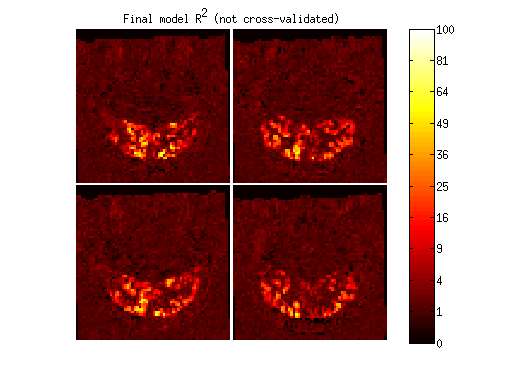
imagesc(imread('example1figures/FinalModel.png'),[0 255]);
colormap(hot);
axis equal tight off;
cb = colorbar;
set(cb,'YTick',linspace(0,255,11),'YTickLabel',round((0:.1:1).^2 * 100));
title('Final model R^2 (not cross-validated)');

% 'NoisePool.png' shows which voxels were used for the noise pool.  Assuming
% the default parameters, the noise pool consists of voxels whose (1) mean
% intensity is greater than one-half of the 99th percentile of mean intensity
% values and (2) cross-validated R^2 value is less than 0%.  Notice that
% the noise pool omits voxels near the top of the slice because the raw
% signal level is relatively low there (due to the distance from the RF coil).
figure;
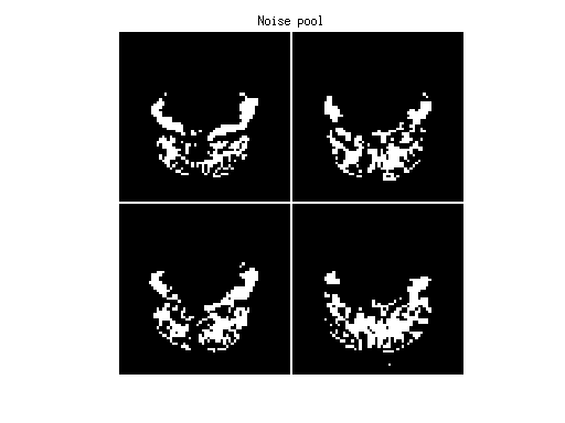
imagesc(imread('example1figures/NoisePool.png'),[0 255]);
colormap(gray);
axis equal tight off;
title('Noise pool');

% 'HRF.png' shows the initial HRF guess (red) and the final HRF estimate (blue).
% Full flexibility is given to the HRF estimate, so the noisiness of the HRF
% estimate gives an indication of the SNR level in the data.  In this case,
% the HRF estimate looks very nice, suggesting that the data have good SNR.
% The first point in the HRF coincides with the onset of a condition (which is
% denoted by 1s in the design matrix).  The granularity of the HRF reflects
% the sampling rate (TR) of the data.
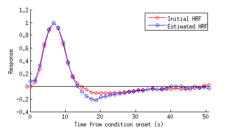
figure;
imageactual('example1figures/HRF.png');

% 'PCcrossvalidationXX.png' shows cross-validated R^2 values corresponding
% to different numbers of PCs.  The color range is 0% to 100%.  Here we show
% the initial model (no PCs) and the final model (number of PCs selected by
% the code).  Notice that because of cross-validation, most voxels are black,
% indicating cross-validated R^2 values that are 0% or less.  Also, notice
% that there is some gain in cross-validation performance in the middle of the
% slices.  The most effective way to view and interpret these figures
% is to flip between them in quick succession, and this is easiest to do
% in your operating system (not in MATLAB).
figure;
set(gcf,'Units','points','Position',[100 100 900 325]);
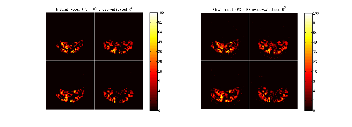
subplot(1,2,1);
imagesc(imread('example1figures/PCcrossvalidation00.png'),[0 255]);
colormap(hot);
axis equal tight off;
cb = colorbar;
set(cb,'YTick',linspace(0,255,11),'YTickLabel',round((0:.1:1).^2 * 100));
title('Initial model (PC = 0) cross-validated R^2');
subplot(1,2,2);
imagesc(imread(sprintf('example1figures/PCcrossvalidation%02d.png',results.pcnum)));
colormap(hot);
axis equal tight off;
cb = colorbar;
set(cb,'YTick',linspace(0,255,11),'YTickLabel',round((0:.1:1).^2 * 100));
title(sprintf('Final model (PC = %d) cross-validated R^2',results.pcnum));

% 'PCscatterXX.png' shows scatter plots of the cross-validation performance of the
% initial model (no PCs) against the performance of individual models with
% different numbers of PCs.  Here we show the scatter plot corresponding to
% the final model (number of PCs selected by the code).  Voxels that were
% used to determine the optimal number of PCs are shown in red; other voxels
% are shown in green.  This figure shows that adding PCs produces a clear and
% consistent improvement in cross-validation performance.
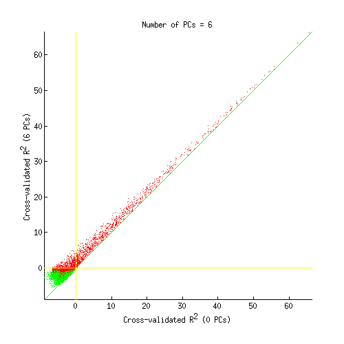
figure;
imageactual(sprintf('example1figures/PCscatter%02d.png',results.pcnum));

% 'PCselection.png' illustrates how the number of PCs was selected.  The median
% cross-validated R^2 value across a subset of the voxels (marked as red
% in the scatter plots) is plotted as a line, and the selected number
% of PCs is marked with a circle.  Assuming the default parameters,
% the code chooses the minimum number of PCs such that the improvement
% relative to the initial model is within 5% of the maximum improvement.
% This is a slightly conservative selection strategy, designed to avoid
% overfitting and to be robust across different datasets.
figure;
imageactual('example1figures/PCselection.png');

Inspect outputs

% The outputs of GLMdenoisedata are contained in
% the variables 'results' and 'denoiseddata'.
% Here we do some basic inspections of the outputs.

% Select a voxel to inspect.  This is done by finding voxels that have
% cross-validated R^2 values between 0% and 5% under the initial model (no PCs),
% and then selecting the voxel that shows the largest improvement when
% using the final model.
ix = find(results.pcR2(:,:,:,1) > 0 & results.pcR2(:,:,:,1) < 5);
improvement = results.pcR2(:,:,:,1+results.pcnum) - results.pcR2(:,:,:,1);
[mm,ii] = max(improvement(ix));
ix = ix(ii);
[xx,yy,zz] = ind2sub(results.inputs.datasize{1}(1:3),ix);

% Inspect amplitude estimates for the example voxel.  The first row shows results
% obtained from the GLMdenoisedata call that does not involve global noise regressors;
% the second row shows results obtained from the regular GLMdenoisedata call.
% The left panels show amplitude estimates from individual bootstraps, whereas
% the right panels show the median and 68% interval across bootstraps (this
% corresponds to the final model estimate and the estimated error on the
% estimate, respectively).
figure;
set(gcf,'Units','points','Position',[100 100 700 500]);
for p=1:2
  if p==1
    ampboots = squeeze(resultsALT.models{2}(xx,yy,zz,:,:));  % conditions x boots
    amp = flatten(resultsALT.modelmd{2}(xx,yy,zz,:));        % 1 x conditions
    ampse = flatten(resultsALT.modelse{2}(xx,yy,zz,:));      % 1 x conditions
  else
    ampboots = squeeze(results.models{2}(xx,yy,zz,:,:));     % conditions x boots
    amp = flatten(results.modelmd{2}(xx,yy,zz,:));           % 1 x conditions
    ampse = flatten(results.modelse{2}(xx,yy,zz,:));         % 1 x conditions
  end
  n = length(amp);
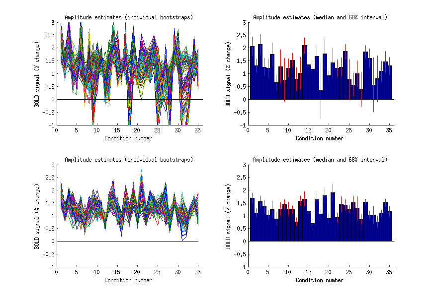
  subplot(2,2,(p-1)*2 + 1); hold on;
  plot(ampboots);
  straightline(0,'h','k-');
  xlabel('Condition number');
  ylabel('BOLD signal (% change)');
  title('Amplitude estimates (individual bootstraps)');
  subplot(2,2,(p-1)*2 + 2); hold on;
  bar(1:length(amp),amp,1);
  errorbar2(1:length(amp),amp,ampse,'v','r-');
  if p==1
    ax = axis; axis([0 n+1 ax(3:4)]); ax = axis;
  end
  xlabel('Condition number');
  ylabel('BOLD signal (% change)');
  title('Amplitude estimates (median and 68% interval)');
end
for p=1:2
  subplot(2,2,(p-1)*2 + 1); axis(ax);
  subplot(2,2,(p-1)*2 + 2); axis(ax);
end

% Compare SNR before and after the use of global noise regressors.
% To focus on voxels that related to the experiment, we select voxels with
% cross-validated R^2 values that are greater than 0% under the initial model.
% To ensure that the SNR values reflect only changes in the noise level,
% we ignore the SNR computed in each individual GLMdenoisedata call and
% re-compute SNR, holding the numerator (the signal) constant across the
% two calls.  (Note: GLMdenoisedata automatically writes out a figure that
% shows a before-and-after SNR comparison (SNRcomparebeforeandafter.png).
% What is shown in this script does the comparison manually just for sake
% of example.)
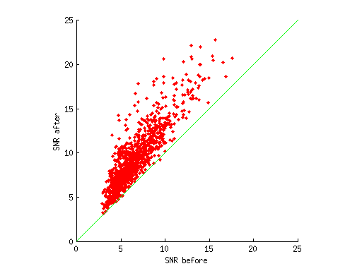
ok = results.pcR2(:,:,:,1) > 0;
signal = mean([results.signal(ok) resultsALT.signal(ok)],2);
snr1 = signal ./ resultsALT.noise(ok);
snr2 = signal ./ results.noise(ok);
figure; hold on;
scatter(snr1,snr2,'r.');
ax = axis;
mx = max(ax(3:4));
axissquarify;
axis([0 mx 0 mx]);
xlabel('SNR before');
ylabel('SNR after');

% An alternative to using the GLM estimates provided by GLMdenoisedata is
% to use 'denoiseddata', which contains the original time-series data but
% with the component of the data that is estimated to be due to the global
% noise regressors subtracted off.  Here we inspect the denoised data for
% the same example voxel examined earlier.  Note that the data components
% that are present in 'denoiseddata' can be customized (see opt.denoisespec
% in GLMdenoisedata.m).  The default parameters leave in the estimated baseline
% signal drift, which explains the drift in the plotted time-series.
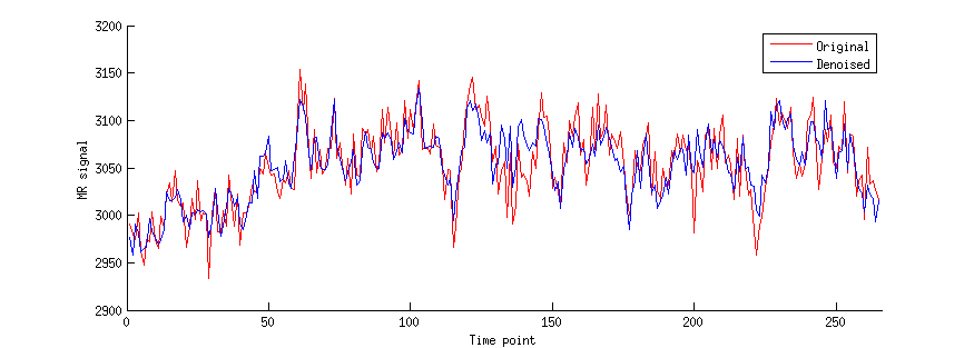
figure; hold on;
set(gcf,'Units','points','Position',[100 100 700 250]);
data1 = flatten(data{1}(xx,yy,zz,:));
data2 = flatten(denoiseddata{1}(xx,yy,zz,:));
n = length(data1);
h1 = plot(data1,'r-');
h2 = plot(data2,'b-');
ax = axis; axis([0 n+1 ax(3:4)]);
legend([h1 h2],{'Original' 'Denoised'});
xlabel('Time point');
ylabel('MR signal');

Published with MATLAB® R2012b